Session 19 (CFM2103)
19.1 Agenda
In this session we are going to revisit some of the concepts discussed in the previous lectures.
This is a revision session to help you complete the forthcoming assignment (the last piece of coursework).
The agenda for this session is split into two main topics that are listed below:
- Initial-value problems (for first-order ODEs)
- Integration
We are going to be mainly interested in reviewing the basic concepts, in discussing some aspects of the numerical implementation using Python, and the testing of the various relevant numerical codes. Everything we do here will be based on procedural programming (i.e., we are going to use functions to achieve our various goals vis-a-vis the aforementioned topics).
19.2 Initial-Value Problems
An initial-value problem consists of an ODE together with an initial condition.
The ODE is typically of the form:
\begin{equation*}
\frac{dy}{dx} = f(x, y)\,.
\label{ec:1} \tag{1}
\end{equation*}
In this equation $f(x, y)$ is a given function of two variables, while $y=y(x)$ is the unknown function that depends on $x$. Note that \eqref{ec:1} can also be cast in the longer form
$$
y'(x) = f(x, y(x))
$$
where we are now using the dash-notation to indicate the derivative of $y$ with respect to $x$.
Solving such a differential equation amounts to finding an expression for the unknown function. This is possib le only in a limited number of cases; separable ODEs can be solved in closed form, while linear ODEs can be reduced to a separable one by using an appropriate integrating factor.
Examples:
1).
$$
\frac{dy}{dx} = 1+y^2\quad\Longrightarrow\quad \frac{dy}{1+y^2}=dx\quad \mbox{(separable)}
$$
2).
$$
\frac{dy}{dx} = x+y\quad\Longrightarrow\quad \frac{dy}{dx}-y = x\quad\mbox{(linear)}
$$
3).
$$
\frac{dy}{dx} = x^2+y^3\quad \mbox{(no analytic solution)}
$$
In these examples the right-hand side corresponds to the obvious functions:
- Ex. 1: $f(x,y) = 1+y^2$.
- Ex. 2: $f(x,y) = x+y$.
- Ex. 3: $f(x,y) = x^2+y^3$.
The solution of a first-order ODE will always depend on one arbitrary constant. Hence, the equations mentioned above do not have just one solution, but an entire family of solutions.
EXAMPLE:
Take the equation in Ex. 2 above. It's a linear equation that is readily solved to give
\begin{equation*}
y(x) = -x - 1 + C e^x \qquad\mbox{(for some constant $C\in\mathbb{R}$)}\,.
\label{ec:2} \tag{2}
\end{equation*}
The constant $C$ is fixed by prescribing what the value of $y(x)$ must be at some point, $x_0$ (say). That is, we are usually interested in the solutions of an ODE that satisfy the additional condition
\begin{equation*}
y(x_0) = y_0\,,
\label{ec:3} \tag{3}
\end{equation*}
where $x_0$ and $y_0$ are given numbers. This additional constraint is known as an initial condition.
Typically, if an initial condition like \eqref{ec:3} is specified, we are interested in finding the values of the function $y(x)$ for $x>x_0$.
EXAMPLE:
If in Ex.2 above we want the solution that satisfies $y(0)=1$, we can use \eqref{ec:3} to obtain $C=2$, so the solution of our initial-value problem will then be
$$
y(x) = -x - 1+2e^x\,.
$$
Note that this expression is a function of $x$ only.
"""
plot of the solution of the linear IVP from Ex.2 with the
initial condition y(0) = 1
"""
%matplotlib notebook
from matplotlib import pyplot as plt
import numpy as np

xmax = 7
x1 = np.linspace(0, xmax, 1000)
x2 = np.linspace(0, xmax, 10)
y1 = -x1 - 1 + 2*np.exp(x1)
y2 = -x2 - 1 + 2*np.exp(x2)
plt.plot(x1,y1,'--b', x2, y2, 'or')
#plt.plot(x2,y2,'or')
plt.xlabel('x')
plt.ylabel('y')
plt.show()

19.3 Numerical approximations for IVPs
Numerical approximations of differential equations are based on replacing the continuous independent variable $x$ with a set of discrete points. This is referred to as a mesh or grid.
A mesh can be coarse or fine, depending on the number of points it contains.
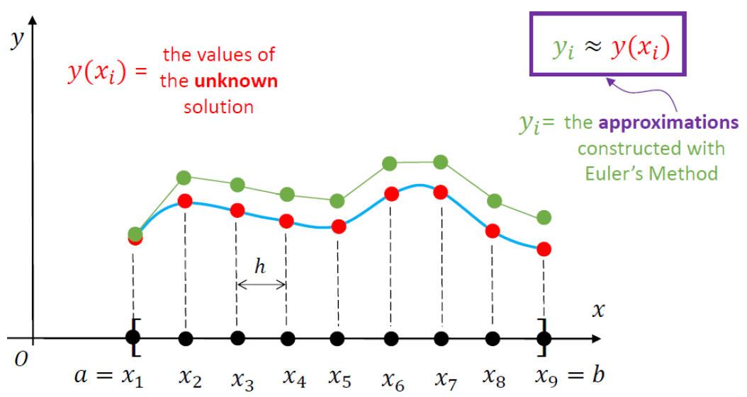
The goal of any numerical scheme for solving a given IVP consists in finding approximations for the
values of the unknown function $y(x)$ at the points of the mesh.
The sketch included below illustrates the notation associated with such a numerical approximation.
(You may want to revisit Session 8 to jog your memory).
19.3.1 Forward Euler
This is the simplest numerical scheme for solving differential equations.
\begin{gather*}
y'(x) = f(x, y(x)),\qquad a\leq x \leq b\\
y(a) = y_0\quad\mbox{(given)}
\end{gather*}
The first step is to consider a uniform mesh over $[a,b]$,
$$
a = x_0 < x_1 < x_2 < ... < x_{n-1} < x_n = b\,,\qquad x_j = a + j h\,,
$$
where
$$
h = \frac{b-a}{n}\quad \mbox{(represents the mesh step size)}\,.
$$
The key idea in this solution strategy (F.E.) is to approximative the derivative
of our differential equation on the mesh. Before we examine that in detail, you
may recall that
$$
y'(x) = \lim_{\Delta x \to 0}\frac{y(x+\Delta x)-y(x)}{\Delta x}\quad\Longrightarrow\quad
y'(x)\simeq \frac{y(x+\Delta x)-y(x)}{\Delta x}\,,
$$
which is true if $|\Delta x|$ is very small (i.e., close to zero). With this in mind we can then write
\begin{equation*}
y(x+\Delta x) = y(x)+y'(x)\Delta x\,,
\label{ec:4} \tag{4}
\end{equation*}
where I replaced "$\simeq$" with the equality sign "$=$".
In equation \eqref{ec:4} we replace $x\to x_j$ and $\Delta x\to h$, to get
\begin{equation*}
y(x_j + h) = y(x_j) + hy'(x_j)\,.
\label{ec:5} \tag{5}
\end{equation*}
If in the original differential equation we set $x\to x_j$, we obtain
\begin{equation*}
y'(x_j) = f(x_j, y(x_j))\,.
\label{ec:6} \tag{6}
\end{equation*}
Combining \eqref{ec:5} and \eqref{ec:6} leads to
$$
y(x_j + h) = y(x_j) + h f(x_j, y(x_j))\,.
$$
Since $y(x_j + h) = y(x_{j+1})\simeq y_{j+1}$ and $y(x_j)\simeq y_j$, the last equation can be cast in the form
\begin{equation*}
y_{j+1} = y_j + hf(x_j, y_j)\qquad\mbox{for}\quad j=0,1,2,\dots, (n-1)
\label{ec:7} \tag{7}
\end{equation*}
Equation \eqref{ec:7} is a recurrence relation that represents the
Forward Euler finite-difference scheme for finding
a numerical approximation of the original initial-value problem.
This is how it works: we set $j=0$, then $j=1$, and so on.
\begin{alignat*}{1}
&y_1 = y_0 + hf(x_0, y_0)\qquad (y_0\mbox{ is given; so are $h$ and $f(x,y)$})\\[0.2cm]
&y_2 = y_1 + hf(x_1, y_1)\\[0.2cm]
&y_3 = y_2 + hf(x_2, y_2)\\[0.2cm]
&y_4 = y_3 + hf(x_3, y_3)\\[0.2cm]
&\dots \mbox{ ETC.}
\end{alignat*}
Numerical Implementation
INPUT :
* f(x, y) = RHS of the ODE.
* a, b    = endpoints of the x-range.
* n       = related to the number of points in the mesh.
Once you have the above you can go on and define h as well as the mesh (that has to be stored in a numpy array).
We can also specify h, as in the implementation below. Note that in this case the step size of the last step won't be the same as h.
OUTPUT :
* a numpy array containing the values of the approximations obtained by using
the above recurrence relation.import numpy as np
def solverFE(f, x, y, xstop, h):
'''Simple Forward Euler integrator '''
# initialise the storage for the solution:
xvals = []
yvals = []
#
# add the initial condition:
xvals.append(x)
yvals.append(y)
while x < xstop:
h = min(h, xstop - x)
y = y + h*f(x, y)
x = x + h
xvals.append(x)
yvals.append(y)
return np.array(xvals), np.array(yvals)
# A very simple check for the above function
# We are just plotting the solution that is computed
# Recall that this is Ex.2 above

%matplotlib notebook
from matplotlib import pyplot as plt

# This is the right-hand side of the ODE:
def f(x, y):
    return x + y

# Inputs:
xinit = 0
yinit = 1.0
xstop = 7.0
hs = 0.1

# Call the integrator
xvals, yvals = solverFE(f, xinit, yinit, xstop, hs)

# Plot the solution:
plt.plot(xvals,yvals,'--')
plt.xlabel('x')
plt.ylabel('y')
plt.show()

The above lines of code are simply used to check that our code runs smoothly and produces some output that can be plotted as seen above. However, this is hardly a test of the accuracy of our code.
To test an initial-value solver we have several options:
- If an analytical solution is available, we can check the numerically computed approximation against the exact solution. This comparison can be in the form of a plot that contains both sets of data, although such an approach fails to give us a precise indication of the absolute and relative errors (A.E. and R.E., respectively).
- If an analytical solution is not readily available we can explore what happens if *h* (the stepsize) is decreased -- in principle, both A.E. and R.E. must go down.
# A very simple TEST for the above function
# We are running the code with 4 different values of h
# and then plot the solutions
# Recall that this is Ex.2 above

%matplotlib notebook
from matplotlib import pyplot as plt

# This is the right-hand side of the ODE:
def f(x, y):
    return x + y

# Inputs:
xinit = 0
yinit = 1.0
xstop = 3.0
hvals = [0.5, 0.05, 0.001, 0.0001]  #stepsize values used

# Initialize lists for storing the numerical results:
xvals = []
yvals = []
# Call the integrator (Forward Euler):
for h in hvals:
    xval, yval = solverFE(f, xinit, yinit, xstop, h)
    xvals.append(xval)
    yvals.append(yval)

# Plot the solutions obtained
# The last two curves overlap -- you must zoom in
#                    to convince yourself of this
mystring = ''
lines = []
labels = []
for i in range(4):
    # Plot the solution:
    lin, = plt.plot(xvals[i],yvals[i],'--')
    lines.append(lin)
    mystring = 'Stepsize: ' + str(hvals[i])
    labels.append(mystring)

plt.legend(lines, labels)
plt.xlabel('x')
plt.ylabel('y')
plt.show()

Recall that we have the analytical solution for this test problem, so we can actually compute the A.E. and R.E. for different meshes. The code included below uses the same four stepsize values as above, but we produce plots for A.E. and R.E., as explained in the comments.
# A simple TEST for the above solver function
# We are running the code with 4 different values of h,
# compute the A.E. and R.E. based on the EXACT SOLUTION
# (which happens to be available in this case), and then
# plot this using matplotlib.
# Recall that this is Ex.2 above

%matplotlib notebook
from matplotlib import pyplot as plt

# This is the right-hand side of the ODE:
def f(x, y):
    return x + y

# Write a function to evaluate the exact solution:
def y_exact(x):
    return -x-1 + 2*np.exp(x)

# Inputs:
xinit = 0
yinit = 1.0
xstop = 3.0
hvals = [0.5, 0.05, 0.001, 0.0001]  #stepsize values used


# Initialize lists for storing the numerical results:
xvals = []
AEvals = []
REvals = []
# Call the integrator (Forward Euler):
for h in hvals:
    xval, yval = solverFE(f, xinit, yinit, xstop, h)
    xvals.append(xval)
    ytmp = y_exact(xval)
    # Compute A.E. and R.E. and store them:
    absval = np.abs(yval - ytmp)
    relval = np.true_divide(absval, np.abs(ytmp))
    AEvals.append(absval)
    REvals.append(relval)

fig, axs = plt.subplots(1,2)
fig.tight_layout(pad=5)
fig.suptitle('Absolute and Relative error for Forward Euler')
for j in range(2,4):
    axs[0].plot(xvals[j], AEvals[j])
    axs[1].plot(xvals[j], REvals[j])

#for ax in axs.flat:
#    print(ax)
axs[0].set(xlabel='x', ylabel= 'A.E.')#; axs[0].axis('square')
axs[1].set(xlabel='x', ylabel= 'R.E.')#; axs[1].axis('square')

plt.show()

The function 'solverFE(....)' can be used to solve systems of first-order ODEs. On several occasions we have already seen that higher-order differential equations can be re-arranged in such a form. We illustrate how this works for the second-order differential equation
$$
y'' = -0.1y' - x\,,\qquad 0\leq x \leq 2\,,
$$
subject to the initial conditions
$$
y(0) = 0\,,\qquad y'(0) = 1\,.
$$
The exact solution can be shown to be
$$
y(x) = 100x - 5x^2 + 990(e^{-0.1 x} - 1)\,.
$$
By introducing the notation
$$
y_0 = y\qquad\mbox{and}\qquad y_1 = y',
$$
we get
$$
\frac{d{\mathbf{y}}}{dx} = \mathbf{f}(x, \mathbf{y})\,,\qquad 0\leq x \leq 2\,,
$$
where
$$
\mathbf{f}(x,\mathbf{y}) = \begin{bmatrix}
y_1\\[0.2cm]
-0.1y_1 - x
\end{bmatrix}\;,\qquad
\mathbf{y}(0) = \begin{bmatrix}
0\\[0.2cm]
1
\end{bmatrix}\;.
$$
This is a vector first-order initial-value problem; that is, the unknown function is the vector
$\mathbf{y}$. The Python code below solves this IVP and compares the result with the analytic solution stated above.
%matplotlib notebook
import numpy as np
from matplotlib import pyplot as plt

def f(x, y):
    # We need a numpy array to store the value of the function
    # at a given x and y (because we are dealing with a VECTOR ode)
    f = np.zeros(2)
    f[0] = y[1]
    f[1] = -0.1*y[1] - x
    return f

# Inputs:
xinit = 0
yinit = np.array([0.0, 1.0])
xstop = 2.0   # want solution for xinit<=x<=xstop
h = 0.0001    # stepsize value used

yval = np.array([0.0, 0.0]) # to store the y-output of solverFE
# Call the integrator (Forward Euler):
xval, yval = solverFE(f, xinit, yinit, xstop, h)
y_exact = 100.0*xval - 5.0*xval**2 +990.0*(np.exp(-0.1*xval) - 1.0)

# Plot the exact and approximate solutions:
plt.plot(xval, yval[:,0], '-b', xval[::520], y_exact[::520], 'or')
plt.grid(True)
plt.xlabel('x'); plt.ylabel('y')
plt.legend(('Numerical', 'Exact'), loc=0)
plt.show()

19.3.2 Heun's Method
This was studied in Session 7 (which you should review to refresh your memory); the MATLAB implementation of this numerical scheme can be found in heun_example1.m posted on Brightspace.
Recall that this is a predictor-corrector method, which means that the approximation at each step involves a two-stage process:
PREDICTOR STEP:
$$
y_{i+1}^* = y_i + hf(x_i, y_i)
$$
CORRECTOR STEP:
$$
y_{i+1} = y_i + \frac{h}{2}\left[f(x_{i+1}, y_{i+1}^*)+f(x_i, y_i)\right]
$$
You may also recall that this is a second-order method (so it is superior to the Forward Euler strategy, which is only a first-order method). In particular, this means that you won't have to consider a very small stepsize in order to obtain a decent approximation.
#
# Numerical implementation of Heun's method
#
from __future__ import print_function
import numpy as np

def solverHEUN(f, x, y, b, h):
    # Create empty lists to store the x and y-values:
    X = []
    Y = []
    # Before the iteration starts, add x0 and y0 to the lists:
    X.append(x)
    Y.append(y)
    # Here starts the main iteration.
    # At each step the stepsize used will be h,
    #  except when we come to the end of the iteration.
    while x < b:
        h = min(h, b-x)
        ystar = y + h*f(x, y)
        y = y + 0.5*h*(f(x+h, ystar) + f(x, y))
        x = x + h
        X.append(x)
        Y.append(y)
    return np.array(X), np.array(Y)
# A very simple check for the HEUN solver
# We are just plotting the solution that is computed
# and compare it against the exact solution.
# Recall that this is Ex.2 at the top of this notebook

%matplotlib notebook
from matplotlib import pyplot as plt
import numpy as np

# This is the right-hand side of the ODE:
def f(x, y):
    return x + y

# Inputs:
xinit = 0
yinit = 1.0
xstop = 7.0
hs = 0.1       # relativelyt large stepsize

# Call the HEUN integrator
xvals, yvals = solverHEUN(f, xinit, yinit, xstop, hs)
y_exact = -xvals - 1.0 + 2.0*np.exp(xvals)  # exact solution

# Plot both the approximation and the exact solutions:
plt.plot(xvals[::5],yvals[::5],'or', xvals, y_exact,'-b')
plt.xlabel('x')
plt.ylabel('y')
plt.show()

19.4 Integration
This topic was first discussed in Session 4, where you'll find several MATLAB codes that illustrate the computer implementation of several simple methods. We looked at three different strategies for approximating a definite integral:
- The Rectangle Method
- The Trapezium Method
- The Simpson Method
All these methods are concerned with the integral
$$ \int_a^b f(x) dx\,, $$
where $f(x)$ is a given function and $a$ and $b$ are given numbers.
Recall that this integral represents a certain area, as seen in the sketch included below

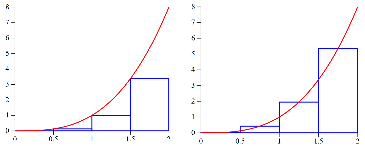
19.4.1. The rectangle Method
This is based on approximating the aforementioned area by using rectangles, as seen below.
We are in control regarding how many rectangles we want to use. It should be intuitively clear that our area is going to be well approximated by having a very large number of such rectangles.
For simplicity, we shall consider a set of equidistant points between $x=a$ and $x=b$:
$$
a = x_0 < x_1 < x_2 <\dots < x_{n-1} < x_n = b\,.
$$
'Equidistant' means that $x_{i+1}-x_i = h$ (constant) for all $i=0,1,\dots, n-1$.

Let's call the various rectangles: $R_0$, $R_1,\,\dots,,R_{n-1}$, and their corresponding areas
$I_0$, $I_1,\,\dots,,I_{n-1}$. Then
\begin{alignat*}{1}
&I_ 0 = (x_1-x_0)f(x_0) = hf(x_0)\,,\\[0.2cm]
&I_1 = (x_2-x_1)f(x_1) = hf(x_1)\,,\\[0.2cm]
&\dots\,,\\[0.2cm]
&I_k = (x_{k+1} - x_k)f(x_k) = hf(x_k)\,,\\[0.2cm]
&\dots\,,\\[0.2cm]
&I_{n-1} = (x_n-x_{n-1})f(x_{n-1}) = hf(x_{n-1})
\end{alignat*}
and hence
\begin{equation*}
\large{\int_a^bf(x)\, dx \simeq I_0 + I_1+ I_2+\dots + I_{n-1}
=h\sum_{k=0}^{n-1} f(x_k)}
\end{equation*}
The absolute error for this approximation is
$$
\large A.E. = \mathcal{O}\left(\frac{(b-a)^2}{2n}\max_{a\leq x\leq b} |f'(x)|\right)
$$
def integrateREC(fname, xmin, xmax, intervals):
    """ Integrate by using the rectangle rule."""
    h = (xmax - xmin) / float(intervals)
    total = 0.0

    # Perform the integration:
    x = xmin
    for interval in range(intervals):
        # Add the area in the trapeziod for this slice:
        total += h * fname(x)

        # Move to the next slice:
        x += h

    return total  # this returns the approx. of the integral
EXAMPLE:
a)
$$
\int_0^{\pi/2} \sin (401 x)\,dx = \frac{1}{401} \simeq 0.00249376
$$
from __future__ import print_function
import numpy as np

def f(x):
    return np.sin(401.0*x)

intervals = [100, 1000, 5000, 10000, 100000]
print("The integral is approximately equal to:")
print(" ")
for interval in intervals:
    print(integrateREC(f, 0, 0.5*np.pi, interval), "\t (n={})".format(interval))
The solutions to CW1 contain worked out examples that illustrate how to test/present your results.
The sample solution posted under Session 4 also contains enough pointers regarding this particular aspect (the difference between MATLAB and Python -- as far as this topic goes, is marginal).
19.4.2 The Trapezium Method
In this case we divide the interval $[a, b]$ into a set of $n$ intervals, each of length $h$. The function whose definite integral we aim to find is approximated by a straight line in each sub-interval, as shown in the sketch below. Hence the area that represents our integral will be approximately equal to the sum of the areas of the trapeziums seen in that sketch.

Let's call the various trapeziums: $T_0$, $T_1,\,\dots,,T_{n-1}$, and their corresponding areas
$I_0$, $I_1,\,\dots,,I_{n-1}$. Then
\begin{alignat*}{1}
&I_ 0 = \frac{1}{2}h[f(x_1)+f(x_0)] \,,\\[0.2cm]
&I_1 = \frac{1}{2}h[f(x_1)+f(x_2)]\,,\\[0.2cm]
&\dots\,,\\[0.2cm]
&I_k = \frac{1}{2}h[f(x_k)+f(x_{k+1})]\,,\\[0.2cm]
&\dots\,,\\[0.2cm]
&I_{n-1} = \frac{1}{2}h[f(x_{n-1})+f(x_n)]
\end{alignat*}
and hence
\begin{alignat*}{1}
\large{\int_a^bf(x)\, dx }&\large{\simeq I_0 + I_1+ I_2+\dots + I_{n-1}}\\[0.1cm]
&\large =\frac{1}{2}h[f(x_0) + 2f(x_1) + 2f(x_2) +\dots + 2f(x_{n-1}) +
f(x_n)]\\[0.1cm]
&\large=\frac{h}{2}[f(x_0) + f(x_n)] + h\sum_{k=1}^{n-1}f(x_k)
\end{alignat*}
The absolute error for this approximation is
$$
\large A.E. = \mathcal{O}\left(\frac{(b-a)^3}{12n^2}\max_{a\leq x\leq b} |f''(x)|\right)
$$
def integrateTRAPZM(fname, xmin, xmax, intervals):
    """ Integrate by using the trapezoid rule."""
    h = (xmax - xmin) / float(intervals)
    total = 0.0

    # Perform the integration:
    x = xmin
    for interval in range(intervals):
        # Add the area in the trapeziod for this slice:
        total += h * (fname(x) + fname(x + h))/float(2.0)

        # Move to the next slice:
        x += h

    return total  # this returns the approx. of the integral
EXAMPLE:
a)
$$
\int_0^\pi e^x\cos x\,dx = -\frac{1}{2}(e^\pi+1)\simeq = -12.070346
$$
from __future__ import print_function
import numpy as np

def f(x):
    return np.exp(x)*np.cos(x)

intervals = [10, 25, 50, 200]
print("The integral is approximately equal to:")
print(" ")
for interval in intervals:
    print(integrateTRAPZM(f, 0, np.pi, interval), "\t (n={})".format(interval))
19.4.3 The Simpson Rule
Again, we start with a set of equidistant points in the interval $[a, b]$.
The idea is to approximate the function $f(x)$ by a parabola on each sub-interval $[x_0, x_2]$,
$[x_2, x_4]$, etc. For this to be possible $n$ must be an EVEN number (any number that is divisible by 2 is an even number).

You have the details of the derivation in Session 4 (lots of details can be found on the internet including YouTube and Khan Academy). Here I'll mention only the final result that is needed for coding this approximation:
$$
\large{{\int_{{a}}^{{b}}}{f{{\left({x}\right)}}}{d}{x}\simeq\frac{{h}}{{3}}{\left({y}_{{0}}+{4}{y}_{{1}}+{2}{y}_{{2}}+{4}{y}_{{3}}+{2}{y}_{{4}}+\ldots+{2}{y}_{{{n}-{2}}}+{4}{y}_{{{n}-{1}}}+{y}_{{n}}\right)}}
$$
where you may recall that
$$
\large{h = (b-a)/n\,.}
$$
Note the pattern of the coefficients:
$$
1, 4, 2, 4, 2, 4, 2, \dots 4, 2, 4, 2, 4, 2, 4, 1
$$
The absolute error for this approximation is
$$
\large A.E. = \mathcal{O}\left(\frac{(b-a)^5}{180n^4}\max_{a\leq x\leq b} |f''''(x)|\right)
$$
def integrateSIMP(f, a, b, N=50):
    """
    Approximate the integral of f(x) from a to b by Simpson's rule.

    INPUTS:
    ----------
    f : function
             of a single variable
    a , b : numbers
        Interval of integration: [a,b]
    N : (even) integer
        Number of subintervals of [a,b]

    OUTPUTS:
    -------
    float
        Approximation of the integral of f(x) over [a, b]
        using Simpson's rule with N subintervals of equal length.
    """
    if N % 2 == 1:
        raise ValueError("N must be an even integer.")
    h = (b-a)/float(N)          # the stepsize
    x = np.linspace(a, b, N+1)   # define the mesh
    y = f(x)
    var = (h/3.0) * np.sum(y[0:-1:2] + 4.0*y[1::2] + y[2::2])  # numerical approx. for integral
    return var
EXAMPLES:
a).
$$
\int_0^\pi\sin(x)\,dx = 2
$$
integrateSIMP(lambda x: np.sin(x), 0.0, np.pi, 30)
b).
$$
\int_0^{\sqrt{\pi}} 2x^2\cos(x^2)\,dx
$$
def f(x):
    return 2.0*(x**2)*np.cos(x**2)

integrateSIMP(f, 0, np.sqrt(np.pi), 60)
c).
$$
\int_0^{\pi/4}\ln(1+\tan x)\,dx
$$
def f(x):
    return np.log(1.0+np.tan(x))

integrateSIMP(f, 0, 0.25*np.pi, 80)
19.4.4. Trapezium Method with control of accuracy
If we want to approximate the value of an integral to within a specified number of significant digits we can keep repeting the process with $h\to h/2$ (which is of course equivalent to doubling the number of 'intervals'). A possible implementation of such a code is included below.
As a typical example, we shall consider the following integral
$$
\int_{\pi/6}^{\pi/2}\sin^2(x)\cos(x)\,dx = \frac{7}{24}\simeq 0.29166666666666\dots\,.
$$
(This integral can be very easily calculated by a simple change of variable.)
from __future__ import print_function
import numpy as np

# define the integrand; you can also use a lambda statement:
def f(x):
    return (np.sin(x)**2)*np.cos(x)
#
#
# specify the integration range as well as the tolerance
# if you want 3 significant digits, TOL = 10**(-3)
# we want 6 significant digits, so TOL = 10**(-6)
TOL = 1.0e-6
a = np.pi/6.0
b = np.pi/2.0
#
# run the Trapezium integrator for intervals = 2
intervals = 2
I_old = 0.0
I_new = integrateTRAPZM(f, a, b, intervals)
#
# keep comparing the difference between the two approximations:
while abs(I_new - I_old) >= TOL:
    I_old = I_new # save the I_new calculated at the previous step
    intervals = 2*intervals  # double the number of sub-intervals
    I_new = integrateTRAPZM(f, a, b, intervals) # find the new approximation
#
# when we break out of the loop I_new will contain
# the desired result:
print("Integral =", I_new)
print("Number of intervals =", intervals)
19.5 The Midpoint Rule
This is a version of the Rectangle Method (more or less). It is based on approximating the area mentioned above by using a special choice of rectangles. In particular, the height of these rectangles corresponds to
$$
f(x_{i}^*)\,,
$$
where
$$
x_i^* = \frac{1}{2}(x_i+x_{i+1})\quad\mbox{is the midpoint of the interval}\qquad (x_i, x_{i+1})
$$
for $i=0,1,2\,\dots, (n-1)$.
Let's call the various rectangles: $R_0$, $R_1,\,\dots,,R_{n-1}$, and their corresponding areas
$I_0$, $I_1,\,\dots,,I_{n-1}$. Then
\begin{alignat*}{1}
&I_ 0 = (x_1-x_0)f(x_0^*) = hf\left(\frac{x_0+x_1}{2}\right)\,,\\[0.2cm]
&I_1 = (x_2-x_1)f(x_1^*) = hf\left(\frac{x_1+x_2}{2}\right)\,,\\[0.2cm]
&\dots\,,\\[0.2cm]
&I_k = (x_{k+1} - x_k)f(x_k^*) = hf\left(\frac{x_k+x_{k+1}}{2}\right)\,,\\[0.2cm]
&\dots\,,\\[0.2cm]
&I_{n-1} = (x_n-x_{n-1})f(x_{n-1}^*) = hf\left(\frac{x_{n-1}+x_n}{2}\right)
\end{alignat*}
and hence
\begin{equation*}
\large{\int_a^bf(x)\, dx \simeq I_0 + I_1+ I_2+\dots + I_{n-1}
=h\sum_{k=0}^{n-1} f(x_k^*)}
\end{equation*}
The absolute error for this approximation is
$$
\large A.E. = \mathcal{O}\left(\frac{(b-a)^3}{24n^2}\max_{a\leq x\leq b} |f''(x)|\right)
$$
HOMEWORK:
Write a Python code that implements this method. Test your code on the examples of the various integrals that apear above.